W3:Recurrent Neural Networks for Time Series

Week 3 Recurrent Neural Networks for Time Series

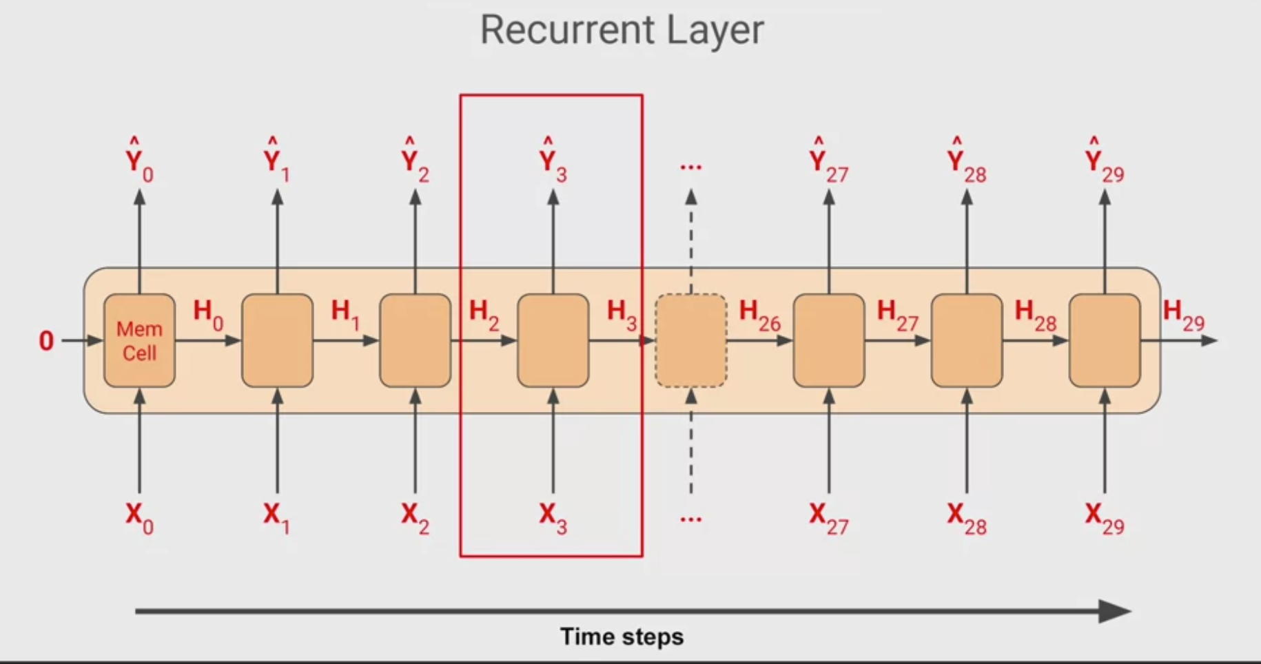
Recurrent Neural networks and Long Short Term Memory networks are really useful to classify and predict on sequential data. This week we’ll explore using them with time series…

Code

import tensorflow as tf
import numpy as np
import matplotlib.pyplot as plt

1 Utilities

Code

def plot_series(time, series, format="-", start=0, end=None):
    """
    Visualizes time series data

    Args:
      time (array of int) - contains the time steps
      series (array of int) - contains the measurements for each time step
      format - line style when plotting the graph
      start - first time step to plot
      end - last time step to plot
    """

    # Setup dimensions of the graph figure
    plt.figure(figsize=(10, 6))
    
    if type(series) is tuple:

      for series_num in series:
        # Plot the time series data
        plt.plot(time[start:end], series_num[start:end], format)

    else:
      # Plot the time series data
      plt.plot(time[start:end], series[start:end], format)

    # Label the x-axis
    plt.xlabel("Time")

    # Label the y-axis
    plt.ylabel("Value")

    # Overlay a grid on the graph
    plt.grid(True)

    # Draw the graph on screen
    plt.show()

def trend(time, slope=0):
    """
    Generates synthetic data that follows a straight line given a slope value.

    Args:
      time (array of int) - contains the time steps
      slope (float) - determines the direction and steepness of the line

    Returns:
      series (array of float) - measurements that follow a straight line
    """

    # Compute the linear series given the slope
    series = slope * time

    return series

def seasonal_pattern(season_time):
    """
    Just an arbitrary pattern, you can change it if you wish
    
    Args:
      season_time (array of float) - contains the measurements per time step

    Returns:
      data_pattern (array of float) -  contains revised measurement values according 
                                  to the defined pattern
    """

    # Generate the values using an arbitrary pattern
    data_pattern = np.where(season_time < 0.4,
                    np.cos(season_time * 2 * np.pi),
                    1 / np.exp(3 * season_time))
    
    return data_pattern

def seasonality(time, period, amplitude=1, phase=0):
    """
    Repeats the same pattern at each period

    Args:
      time (array of int) - contains the time steps
      period (int) - number of time steps before the pattern repeats
      amplitude (int) - peak measured value in a period
      phase (int) - number of time steps to shift the measured values

    Returns:
      data_pattern (array of float) - seasonal data scaled by the defined amplitude
    """
    
    # Define the measured values per period
    season_time = ((time + phase) % period) / period

    # Generates the seasonal data scaled by the defined amplitude
    data_pattern = amplitude * seasonal_pattern(season_time)

    return data_pattern

def noise(time, noise_level=1, seed=None):
    """Generates a normally distributed noisy signal

    Args:
      time (array of int) - contains the time steps
      noise_level (float) - scaling factor for the generated signal
      seed (int) - number generator seed for repeatability

    Returns:
      noise (array of float) - the noisy signal
    """

    # Initialize the random number generator
    rnd = np.random.RandomState(seed)

    # Generate a random number for each time step and scale by the noise level
    noise = rnd.randn(len(time)) * noise_level
    
    return noise

2 Generate the Synthetic Data

Code

# Parameters
time = np.arange(4 * 365 + 1, dtype="float32")
baseline = 10
amplitude = 40
slope = 0.05
noise_level = 5

# Create the series
series = baseline + trend(time, slope) + seasonality(time, period=365, amplitude=amplitude)

# Update with noise
series += noise(time, noise_level, seed=42)

# Plot the results
plot_series(time, series)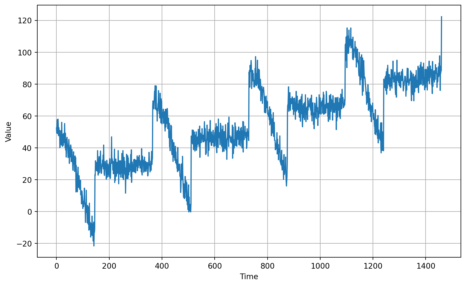

3 Split the Dataset

Code

# Define the split time
split_time = 1000

# Get the train set 
time_train = time[:split_time]
x_train = series[:split_time]

# Get the validation set
time_valid = time[split_time:]
x_valid = series[split_time:]

4 Prepare Features and Labels

Code

# Parameters
window_size = 20
batch_size = 32
shuffle_buffer_size = 1000

Code

def windowed_dataset(series, window_size, batch_size, shuffle_buffer):
    """Generates dataset windows

    Args:
      series (array of float) - contains the values of the time series
      window_size (int) - the number of time steps to include in the feature
      batch_size (int) - the batch size
      shuffle_buffer(int) - buffer size to use for the shuffle method

    Returns:
      dataset (TF Dataset) - TF Dataset containing time windows
    """
  
    # Generate a TF Dataset from the series values
    dataset = tf.data.Dataset.from_tensor_slices(series)
    
    # Window the data but only take those with the specified size
    dataset = dataset.window(window_size + 1, shift=1, drop_remainder=True)
    
    # Flatten the windows by putting its elements in a single batch
    dataset = dataset.flat_map(lambda window: window.batch(window_size + 1))

    # Create tuples with features and labels 
    dataset = dataset.map(lambda window: (window[:-1], window[-1]))

    # Shuffle the windows
    dataset = dataset.shuffle(shuffle_buffer)
    
    # Create batches of windows
    dataset = dataset.batch(batch_size).prefetch(1)
    
    return dataset

Code

# Generate the dataset windows
dataset = windowed_dataset(x_train, window_size, batch_size, shuffle_buffer_size)

5 define RNN model

Code

# Build the Model
model_tune = tf.keras.models.Sequential([
  tf.keras.layers.Lambda(lambda x: tf.expand_dims(x, axis=-1),
                      input_shape=[window_size]),
  tf.keras.layers.SimpleRNN(40, return_sequences=True),
  tf.keras.layers.SimpleRNN(40),
  tf.keras.layers.Dense(1),
  tf.keras.layers.Lambda(lambda x: x * 100.0)
])

# Print the model summary
model_tune.summary()

Model: "sequential"

┏━━━━━━━━━━━━━━━━━━━━━━━━━━━━━━━━━┳━━━━━━━━━━━━━━━━━━━━━━━━┳━━━━━━━━━━━━━━━┓
┃ Layer (type)                    ┃ Output Shape           ┃       Param # ┃
┡━━━━━━━━━━━━━━━━━━━━━━━━━━━━━━━━━╇━━━━━━━━━━━━━━━━━━━━━━━━╇━━━━━━━━━━━━━━━┩
│ lambda (Lambda)                 │ (None, 20, 1)          │             0 │
├─────────────────────────────────┼────────────────────────┼───────────────┤
│ simple_rnn (SimpleRNN)          │ (None, 20, 40)         │         1,680 │
├─────────────────────────────────┼────────────────────────┼───────────────┤
│ simple_rnn_1 (SimpleRNN)        │ (None, 40)             │         3,240 │
├─────────────────────────────────┼────────────────────────┼───────────────┤
│ dense (Dense)                   │ (None, 1)              │            41 │
├─────────────────────────────────┼────────────────────────┼───────────────┤
│ lambda_1 (Lambda)               │ (None, 1)              │             0 │
└─────────────────────────────────┴────────────────────────┴───────────────┘

 Total params: 4,961 (19.38 KB)

 Trainable params: 4,961 (19.38 KB)

 Non-trainable params: 0 (0.00 B)

Using Huber loss

Code

# Set the learning rate scheduler
lr_schedule = tf.keras.callbacks.LearningRateScheduler(
    lambda epoch: 1e-8 * 10**(epoch / 20))

# Initialize the optimizer
optimizer = tf.keras.optimizers.SGD(momentum=0.9)

# Set the training parameters
model_tune.compile(loss=tf.keras.losses.Huber(), optimizer=optimizer)

# Train the model
history = model_tune.fit(dataset, epochs=100, callbacks=[lr_schedule],verbose=0)

Code

# Define the learning rate array
lrs = 1e-8 * (10 ** (np.arange(100) / 20))

# Set the figure size
plt.figure(figsize=(10, 6))

# Set the grid
plt.grid(True)

# Plot the loss in log scale
plt.semilogx(lrs, history.history["loss"])

# Increase the tickmarks size
plt.tick_params('both', length=10, width=1, which='both')

# Set the plot boundaries
plt.axis([1e-8, 1e-3, 0, 50])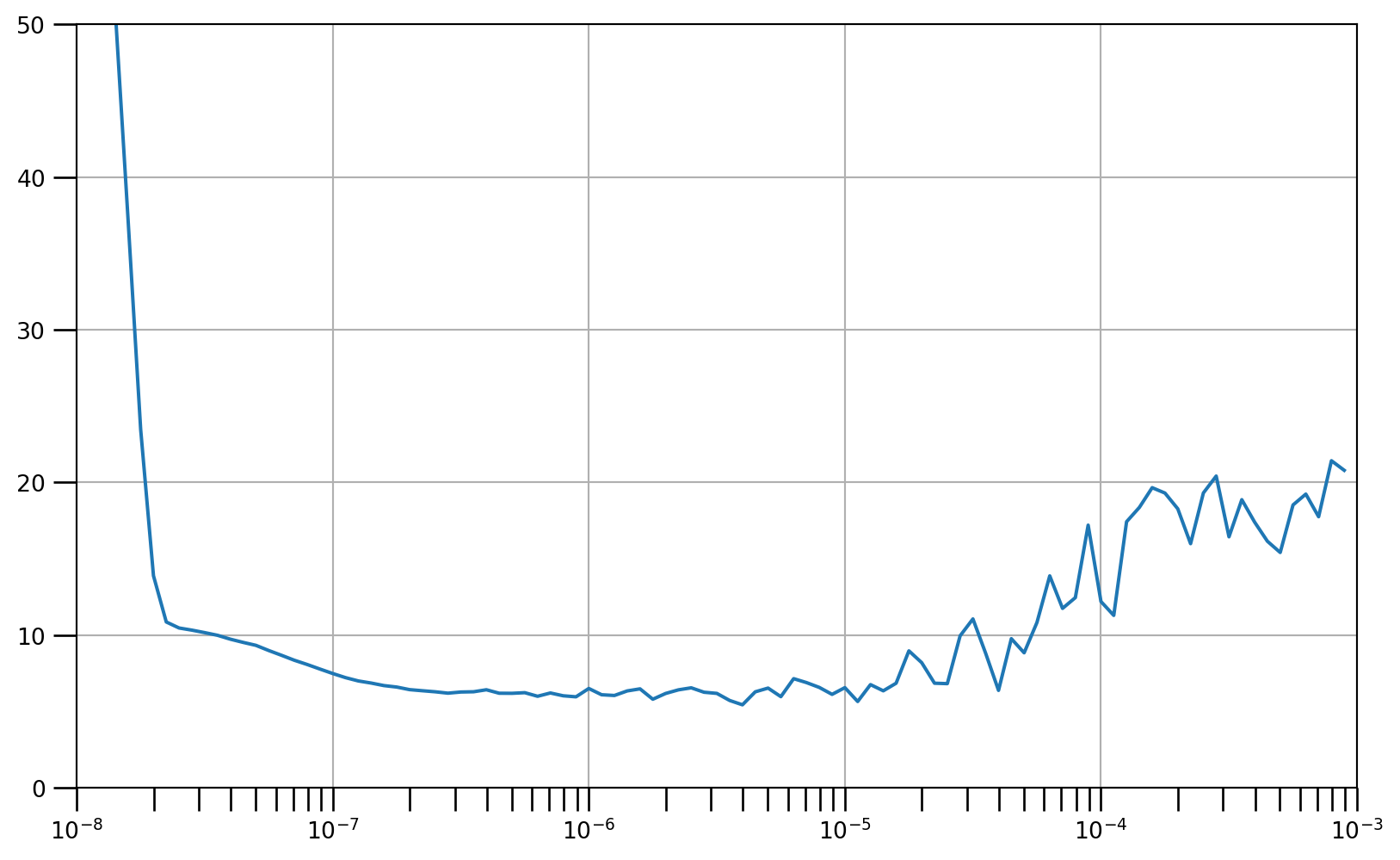

Code

# Set the figure size
plt.figure(figsize=(10, 6))

# Set the grid
plt.grid(True)

# Plot the loss in log scale
plt.semilogx(lrs, history.history["loss"])

# Increase the tickmarks size
plt.tick_params('both', length=10, width=1, which='both')

# Set the plot boundaries
plt.axis([1e-7, 1e-4, 0, 20])

6 train model with tunned learning rate

Code

# Build the model
model = tf.keras.models.Sequential([
  tf.keras.layers.Lambda(lambda x: tf.expand_dims(x, axis=-1),
                      input_shape=[window_size]),
  tf.keras.layers.SimpleRNN(40, return_sequences=True),
  tf.keras.layers.SimpleRNN(40),
  tf.keras.layers.Dense(1),
  tf.keras.layers.Lambda(lambda x: x * 100.0)
])

# Set the learning rate
learning_rate = 1e-6

# Set the optimizer 
optimizer = tf.keras.optimizers.SGD(learning_rate=learning_rate, momentum=0.9)

# Set the training parameters
model.compile(loss=tf.keras.losses.Huber(),
              optimizer=optimizer,
              metrics=["mae"])

# Train the model
history = model.fit(dataset,epochs=100,verbose=0)

7 Model Prediction

Code

# Initialize a list
forecast = []

# Reduce the original series
forecast_series = series[split_time - window_size:]

# Use the model to predict data points per window size
for time in range(len(forecast_series) - window_size):
  forecast.append(model.predict(forecast_series[time:time + window_size][np.newaxis]))

# Convert to a numpy array and drop single dimensional axes
results = np.array(forecast).squeeze()

# Plot the results
plot_series(time_valid, (x_valid, results))

Code

def model_forecast(model, series, window_size, batch_size):
    """Uses an input model to generate predictions on data windows

    Args:
      model (TF Keras Model) - model that accepts data windows
      series (array of float) - contains the values of the time series
      window_size (int) - the number of time steps to include in the window
      batch_size (int) - the batch size

    Returns:
      forecast (numpy array) - array containing predictions
    """

    # Generate a TF Dataset from the series values
    dataset = tf.data.Dataset.from_tensor_slices(series)

    # Window the data but only take those with the specified size
    dataset = dataset.window(window_size, shift=1, drop_remainder=True)

    # Flatten the windows by putting its elements in a single batch
    dataset = dataset.flat_map(lambda w: w.batch(window_size))
    
    # Create batches of windows
    dataset = dataset.batch(batch_size).prefetch(1)
    
    # Get predictions on the entire dataset
    forecast = model.predict(dataset)
    
    return forecast

Code

# Reduce the original series
forecast_series = series[split_time - window_size:-1]

# Use helper function to generate predictions
forecast = model_forecast(model, forecast_series, window_size, batch_size)

# Drop single dimensional axis
results = forecast.squeeze()

# Plot the results
plot_series(time_valid, (x_valid, results))

Code

# Compute the MSE and MAE
print(tf.keras.metrics.mean_squared_error(x_valid, results).numpy())

81.265686

Code

print(tf.keras.metrics.mean_absolute_error(x_valid, results).numpy())

6.6564226

8 define LSTM model

clear

Code

tf.keras.backend.clear_session()

Code

# Build the Model
model_tune = tf.keras.models.Sequential([
  tf.keras.layers.Lambda(lambda x: tf.expand_dims(x, axis=-1),
                      input_shape=[window_size]),
    tf.keras.layers.Bidirectional(tf.keras.layers.LSTM(32, return_sequences=True)),
    tf.keras.layers.Bidirectional(tf.keras.layers.LSTM(32, return_sequences=True)),
  tf.keras.layers.Bidirectional(tf.keras.layers.LSTM(32)),
  tf.keras.layers.Dense(1),
  tf.keras.layers.Lambda(lambda x: x * 100.0)
])

# Print the model summary
model_tune.summary()

Model: "sequential"

┏━━━━━━━━━━━━━━━━━━━━━━━━━━━━━━━━━┳━━━━━━━━━━━━━━━━━━━━━━━━┳━━━━━━━━━━━━━━━┓
┃ Layer (type)                    ┃ Output Shape           ┃       Param # ┃
┡━━━━━━━━━━━━━━━━━━━━━━━━━━━━━━━━━╇━━━━━━━━━━━━━━━━━━━━━━━━╇━━━━━━━━━━━━━━━┩
│ lambda (Lambda)                 │ (None, 20, 1)          │             0 │
├─────────────────────────────────┼────────────────────────┼───────────────┤
│ bidirectional (Bidirectional)   │ (None, 20, 64)         │         8,704 │
├─────────────────────────────────┼────────────────────────┼───────────────┤
│ bidirectional_1 (Bidirectional) │ (None, 20, 64)         │        24,832 │
├─────────────────────────────────┼────────────────────────┼───────────────┤
│ bidirectional_2 (Bidirectional) │ (None, 64)             │        24,832 │
├─────────────────────────────────┼────────────────────────┼───────────────┤
│ dense (Dense)                   │ (None, 1)              │            65 │
├─────────────────────────────────┼────────────────────────┼───────────────┤
│ lambda_1 (Lambda)               │ (None, 1)              │             0 │
└─────────────────────────────────┴────────────────────────┴───────────────┘

 Total params: 58,433 (228.25 KB)

 Trainable params: 58,433 (228.25 KB)

 Non-trainable params: 0 (0.00 B)

9 Tune the Learning Rate

using Huber loss

Code

# Set the learning rate scheduler
lr_schedule = tf.keras.callbacks.LearningRateScheduler(
    lambda epoch: 1e-8 * 10**(epoch / 20))

# Initialize the optimizer
optimizer = tf.keras.optimizers.SGD(momentum=0.9)

# Set the training parameters
model_tune.compile(loss=tf.keras.losses.Huber(), optimizer=optimizer)

# Train the model
history = model_tune.fit(dataset, epochs=100, callbacks=[lr_schedule],verbose=0)

Code

# Define the learning rate array
lrs = 1e-8 * (10 ** (np.arange(100) / 20))

# Set the figure size
plt.figure(figsize=(10, 6))

# Set the grid
plt.grid(True)

# Plot the loss in log scale
plt.semilogx(lrs, history.history["loss"])

# Increase the tickmarks size
plt.tick_params('both', length=10, width=1, which='both')

# Set the plot boundaries
plt.axis([1e-8, 1e-3, 0, 30])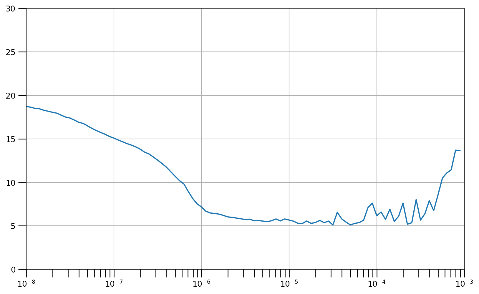

10 train model with tunned learning rate

Code

# Reset states generated by Keras
tf.keras.backend.clear_session()

# Build the model
model = tf.keras.models.Sequential([
  tf.keras.layers.Lambda(lambda x: tf.expand_dims(x, axis=-1),
                      input_shape=[None]),
   tf.keras.layers.Bidirectional(tf.keras.layers.LSTM(32, return_sequences=True)),
  tf.keras.layers.Bidirectional(tf.keras.layers.LSTM(32)),
  tf.keras.layers.Dense(1),
  tf.keras.layers.Lambda(lambda x: x * 100.0)
])

# compile

# Set the learning rate
learning_rate = 2e-6

# Set the optimizer 
optimizer = tf.keras.optimizers.SGD(learning_rate=learning_rate, momentum=0.9)

# Set the training parameters
model.compile(loss=tf.keras.losses.Huber(),
              optimizer=optimizer,
              metrics=["mae"])

# Train
# Train the model
history = model.fit(dataset,epochs=100,verbose=0)

11 Model Prediction

Code

def model_forecast(model, series, window_size, batch_size):
    """Uses an input model to generate predictions on data windows

    Args:
      model (TF Keras Model) - model that accepts data windows
      series (array of float) - contains the values of the time series
      window_size (int) - the number of time steps to include in the window
      batch_size (int) - the batch size

    Returns:
      forecast (numpy array) - array containing predictions
    """

    # Generate a TF Dataset from the series values
    dataset = tf.data.Dataset.from_tensor_slices(series)

    # Window the data but only take those with the specified size
    dataset = dataset.window(window_size, shift=1, drop_remainder=True)

    # Flatten the windows by putting its elements in a single batch
    dataset = dataset.flat_map(lambda w: w.batch(window_size))
    
    # Create batches of windows
    dataset = dataset.batch(batch_size).prefetch(1)
    
    # Get predictions on the entire dataset
    forecast = model.predict(dataset)
    
    return forecast

Code

# Reduce the original series
forecast_series = series[split_time-window_size:-1]

# Use helper function to generate predictions
forecast = model_forecast(model, forecast_series, window_size, batch_size)

# Drop single dimensional axis
results = forecast.squeeze()

# Plot the results
plot_series(time_valid, (x_valid, results))

Code

# Compute the MSE and MAE
print(tf.keras.metrics.mean_squared_error(x_valid, results).numpy())

74.571434

Code

print(tf.keras.metrics.mean_absolute_error(x_valid, results).numpy())

6.1871777

12 13 resource:

https://www.coursera.org/learn/tensorflow-sequences-time-series-and-prediction

https://github.com/https-deeplearning-ai/tensorflow-1-public/tree/main/C4